Anisotropic zinc crystal
In this cookbook (see benchmarks/src/dim2/anisotropic-crystal), we simulate wave propagation through a 2-dimensional anisotropic zinc crystal.
Setting up the workspace
Let’s start by creating a workspace from where we can run this example.
mkdir -p ~/specfempp-examples/anisotropic-crystal
cd ~/specfempp-examples/anisotropic-crystal
We also need to check that the SPECFEM++ executable directory is added to the PATH.
which specfem2d
If the above command returns a path to the specfem2d executable, then the
build directory is added to the PATH. If not, you need to add the executable
directory to the PATH using the following command.
export PATH=$PATH:<PATH TO SPECFEM++ DIRECTORY/bin>
Note
Make sure to replace <PATH TO SPECFEM++ DIRECTORY/bin> with the
actual path to the SPECFEM++ directory on your system.
Now let’s create the necessary directories to store the input files and output artifacts.
mkdir -p OUTPUT_FILES
mkdir -p OUTPUT_FILES/results

touch specfem_config.yaml
touch source.yaml
touch topography_file.dat
touch Par_File
Meshing the domain
Let’s start by defining a mesh with anisotropic domains using the following parameter file.
Parameter file
#-----------------------------------------------------------
#
# Simulation input parameters
#
#-----------------------------------------------------------

# title of job
title                           = Anisotropic Crystal
# parameters concerning partitioning
NPROC                           = 1              # number of processes

# Output folder to store mesh related files
OUTPUT_FILES                   = OUTPUT_FILES

#-----------------------------------------------------------
#
# Mesh
#
#-----------------------------------------------------------

# Partitioning algorithm for decompose_mesh
PARTITIONING_TYPE               = 3              # SCOTCH = 3, ascending order (very bad idea) = 1

# number of control nodes per element (4 or 9)
NGNOD                           = 4

# location to store the mesh
database_filename               = ./OUTPUT_FILES/database.bin

#-----------------------------------------------------------
#
# Receivers
#
#-----------------------------------------------------------


# use an existing STATION file found in ./DATA or create a new one from the receiver positions below in this Par_file
use_existing_STATIONS           = .false.

# number of receiver sets (i.e. number of receiver lines to create below)
nreceiversets                   = 1

# orientation
anglerec                        = 0.d0           # angle to rotate components at receivers
rec_normal_to_surface           = .false.        # base anglerec normal to surface (external mesh and curve file needed)

# first receiver set (repeat these 6 lines and adjust nreceiversets accordingly)
nrec                            = 50             # number of receivers
xdeb                            = 0.05           # first receiver x in meters
zdeb                            = 0.2640         # first receiver z in meters
xfin                            = 0.28           # last receiver x in meters (ignored if only one receiver)
zfin                            = 0.2640         # last receiver z in meters (ignored if only one receiver)
record_at_surface_same_vertical = .false.        # receivers inside the medium or at the surface

# filename to store stations file
stations_filename              = ./OUTPUT_FILES/STATIONS

#-----------------------------------------------------------
#
# Velocity and density models
#
#-----------------------------------------------------------

# number of model materials
nbmodels                        = 1
# available material types (see user manual for more information)
#   acoustic:    model_number 1 rho Vp 0  0 0 QKappa Qmu 0 0 0 0 0 0
#   elastic:     model_number 1 rho Vp Vs 0 0 QKappa Qmu 0 0 0 0 0 0
#   anisotropic: model_number 2 rho c11 c13 c15 c33 c35 c55 c12 c23 c25 0 0 0
#   poroelastic: model_number 3 rhos rhof phi c kxx kxz kzz Ks Kf Kfr etaf mufr Qmu
#   tomo:        model_number -1 0 9999 9999 A 0 0 9999 9999 0 0 0 0 0
1 2 7100. 16.5d10 5.d10 0 6.2d10 0 3.96d10 0 0 0 0 0 0

# external tomography file
TOMOGRAPHY_FILE                 = ./DATA/tomo_file.xyz

# use an external mesh created by an external meshing tool or use the internal mesher
read_external_mesh              = .false.

#-----------------------------------------------------------
#
# PARAMETERS FOR EXTERNAL MESHING
#
#-----------------------------------------------------------

# data concerning mesh, when generated using third-party app (more info in README)
# (see also absorbing_conditions above)
mesh_file                       = ./DATA/Mesh_canyon/canyon_mesh_file   # file containing the mesh
nodes_coords_file               = ./DATA/Mesh_canyon/canyon_nodes_coords_file   # file containing the nodes coordinates
materials_file                  = ./DATA/Mesh_canyon/canyon_materials_file   # file containing the material number for each element
free_surface_file               = ./DATA/Mesh_canyon/canyon_free_surface_file   # file containing the free surface
axial_elements_file             = ./DATA/axial_elements_file   # file containing the axial elements if AXISYM is true
absorbing_surface_file          = ./DATA/Mesh_canyon/canyon_absorbing_surface_file   # file containing the absorbing surface
acoustic_forcing_surface_file   = ./DATA/MSH/Surf_acforcing_Bottom_enforcing_mesh   # file containing the acoustic forcing surface
absorbing_cpml_file             = ./DATA/absorbing_cpml_file   # file containing the CPML element numbers
tangential_detection_curve_file = ./DATA/courbe_eros_nodes  # file containing the curve delimiting the velocity model

#-----------------------------------------------------------
#
# PARAMETERS FOR INTERNAL MESHING
#
#-----------------------------------------------------------

# file containing interfaces for internal mesh
interfacesfile                  = topography_file.dat

# geometry of the model (origin lower-left corner = 0,0) and mesh description
xmin                            = 0.d0           # abscissa of left side of the model
xmax                            = 0.33           # abscissa of right side of the model
nx                              = 60             # number of elements along X

# Stacey ABC
STACEY_ABSORBING_CONDITIONS     = .false.

# absorbing boundary parameters (see absorbing_conditions above)
absorbbottom                    = .false.
absorbright                     = .false.
absorbtop                       = .false.
absorbleft                      = .false.

# define the different regions of the model in the (nx,nz) spectral-element mesh
nbregions                       = 1              # then set below the different regions and model number for each region
# format of each line: nxmin nxmax nzmin nzmax material_number
1 60 1   60 1

#-----------------------------------------------------------
#
# Display parameters
#
#-----------------------------------------------------------

# meshing output
output_grid_Gnuplot             = .false.        # generate a GNUPLOT file containing the grid, and a script to plot it
output_grid_ASCII               = .false.        # dump the grid in an ASCII text file consisting of a set of X,Y,Z points or not
Note the material string used to define an anisotropic velocity model.
70# anisotropic: model_number 2 rho c11 c13 c15 c33 c35 c55 c12 c23 c25 0 0 0
The actual material is then numerically defined in the following line.
731 2 7100. 16.5d10 5.d10 0 6.2d10 0 3.96d10 0 0 0 0 0 0
The material string generates an anisotopic medium with the following properties
Density \(rho = 7100.0 \mathrm{kg}/\mathrm{m}^3\)
\(C_{11} = 16.5 \cdot 10^{10} \mathrm{Pa}\)
\(C_{13} = 5.0 \cdot 10^{10} \mathrm{Pa}\)
\(C_{15} = 0.0 \mathrm{Pa}\)
\(C_{33} = 6.2 \cdot 10^{10} \mathrm{Pa}\)
\(C_{35} = 0.0 \mathrm{Pa}\)
\(C_{55} = 3.96 \cdot 10^{10} \mathrm{Pa}\)
\(C_{12} = 0.0 \mathrm{Pa}\)
\(C_{23} = 0.0 \mathrm{Pa}\)
\(C_{25} = 0.0 \mathrm{Pa}\)
Defining the topography of the domain
Next, as in previous examples, we define the topography of the domain in the
topography_file.dat file. This is very similar to Homogeneous elastic media
with the main difference that this model is much smaller.
#
# number of interfaces
#
2
#
# for each interface below, we give the number of points and then x,z for each point
#
#
# interface number 1 (bottom of the mesh)
#
2
0 0
0.33 0
#
# interface number 2 (topography, top of the mesh)
#
2
    0 0.33
0.33 0.33
#
# for each layer, we give the number of spectral elements in the vertical direction
#
#
# layer number 1 (bottom layer)
#
60
Running xmeshfem2D
To execute the mesher run
xmeshfem2D -p Par_File
Note the path of the database file and a stations file generated after successfully running the mesher.
Defining the source
We define the source location and the source time function in the source file.
number-of-sources: 1
sources:
  - force:
      x : 0.165
      z : 0.165
      source_surf: false
      angle : 0.0
      vx : 0.0
      vz : 0.0
      Ricker:
        factor: 1e10
        tshift: 0.0
        f0: 170000.0
Running the simulation
To run the solver, we first need to define a configuration file
specfem_config.yaml.
## Coupling interfaces have code flow that is dependent on orientation of the interface.
## This test is to check the code flow for horizontal acoustic-elastic interface with acoustic domain on top.

parameters:

  header:
    ## Header information is used for logging. It is good practice to give your simulations explicit names
    title: Homogeneous anisotropic crystal
    # A detailed description for your simulation
    description: |
      Material systems : Elastic Anisotropic domain
      Interfaces : None
      Sources : Force source (1)
      Boundary conditions : Neumann BCs on all edges

  simulation-setup:
    ## quadrature setup
    quadrature:
      quadrature-type: GLL4

    ## Solver setup
    solver:
      time-marching:
        type-of-simulation: forward
        time-scheme:
          type: Newmark
          dt: 55.e-9
          nstep: 1500

    simulation-mode:
      forward:
        writer:
          seismogram:
            format: ascii
            directory: "./OUTPUT_FILES/results"

          display:
            format: PNG
            directory: ./OUTPUT_FILES/results
            field: displacement
            simulation-field: forward
            time-interval: 100

  receivers:
    stations: "./OUTPUT_FILES/STATIONS"
    angle: 0.0
    seismogram-type:
      - displacement
    nstep_between_samples: 1

  ## Runtime setup
  run-setup:
    number-of-processors: 1
    number-of-runs: 1

  ## databases
  databases:
    mesh-database: "./OUTPUT_FILES/database.bin"

  ## Sources
  sources: "./source.yaml"
The solver file is familiar to the previous examples. However, we have added a
display section to generate a wavefield snapshot at every 100th time step.
          display:
            format: PNG
            directory: ./OUTPUT_FILES/results
            field: displacement
            simulation-field: forward
            time-interval: 100
Now we can run the solver using the following command.
specfem2d -p specfem_config.yaml
Visualizing the traces and wavefield
We can plot the traces stored in the OUTPUT_FILES/results directory using
the following python code.
import glob
import os
import numpy as np
import obspy


def get_traces(directory):
    traces = []
    station_name = [
        "S0010",
        "S0020",
        "S0030",
        "S0040",
        "S0050",
    ]
    files = []
    for station in station_name:
        files += glob.glob(directory + f"/??.{station}.S2.BX?.semd")

    ## iterate over all seismograms
    for filename in files:
        station_id = os.path.splitext(filename)[0]
        station_id = station_id.split("/")[-1]
        network, station, location, channel = station_id.split(".")[:4]
        trace = np.loadtxt(filename, delimiter=" ")
        starttime = trace[0, 0]
        dt = trace[1, 0] - trace[0, 0]
        traces.append(
            obspy.Trace(
                trace[:, 1],
                {
                    "network": network,
                    "station": station,
                    "location": location,
                    "channel": channel,
                    "starttime": starttime,
                    "delta": dt,
                },
            )
        )

    stream = obspy.Stream(traces)

    return stream


stream = get_traces("OUTPUT_FILES/results")
stream.select(component="X").plot(size=(1000, 750))
stream.select(component="Z").plot(size=(1000, 750))
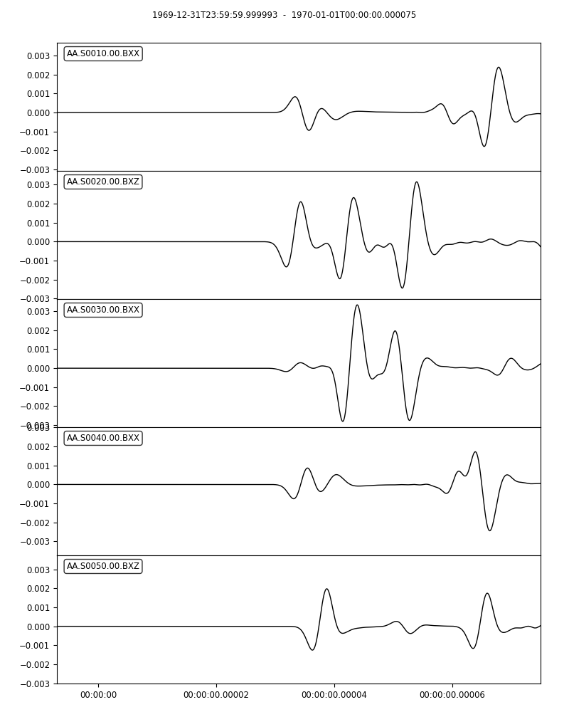
Traces.
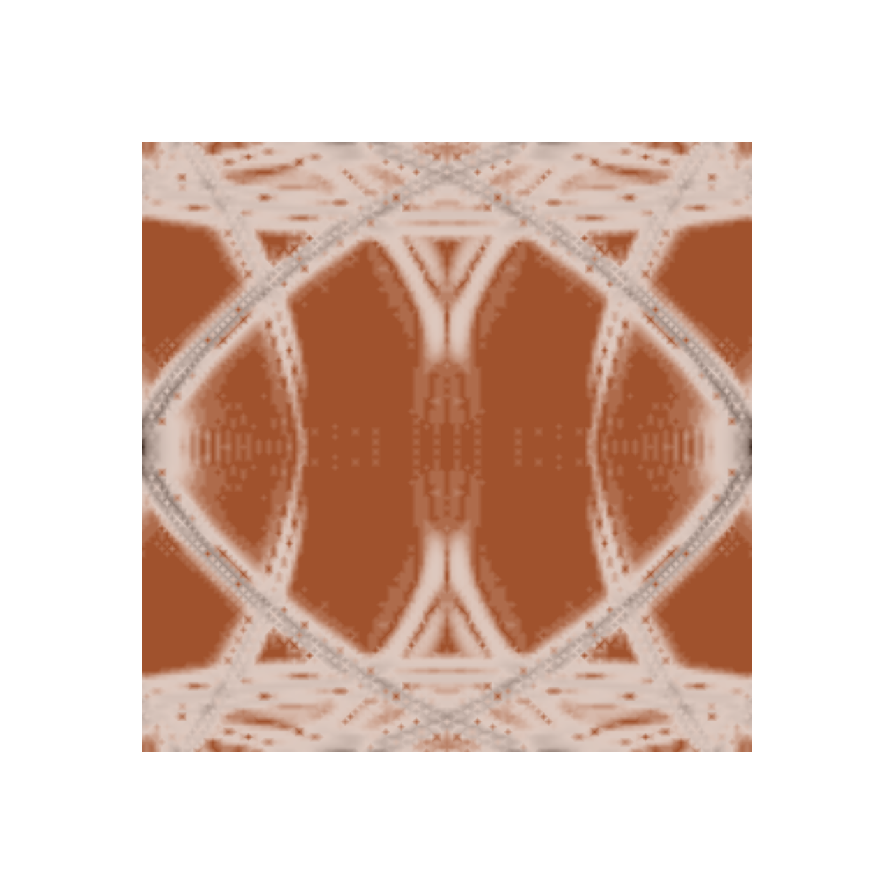
Wavefield snapshot at 1400th time-step.