Adjoint simulations and banana-donut kernels
This example (see benchmarks/src/dim2/Tromp_2005)
demonstrates how to setup forward and adjoint simulations to compute the banana
donut kernels. We will reproduce the results from Fig 9 of Tromp et al. 2005.
Setting up the workspace
Let’s start by creating a workspace from where we can run this example.
mkdir -p ~/specfempp-examples/Tromp_2005
cd ~/specfempp-examples/Tromp_2005
We also need to check that the SPECFEM++ executable directory is added to the
PATH.
which specfem2d
If the above command returns a path to the specfem2d executable, then the
executable directory is added to the PATH. If not, you need to add the
executable directory to the PATH using the following command.
export PATH=$PATH:<PATH TO SPECFEM++ DIRECTORY/bin>
Note
Make sure to replace <PATH TO SPECFEM++ DIRECTORY/bin> with the
actual path to the SPECFEM++ directory on your system.
Now let’s create the necessary directories to store the input files and output artifacts.
mkdir -p OUTPUT_FILES
mkdir -p OUTPUT_FILES/seismograms
mkdir -p OUTPUT_FILES/kernels
mkdir -p OUTPUT_FILES/adjoint_sources

touch forward_config.yaml
touch forward_sources.yaml
touch adjoint_config.yaml
touch adjoint_sources.yaml
touch topography_file.dat
touch Par_File
Setting up the forward simulation
Lets start by setting up a forward simulation as we did in the previous notebooks. As before, we will need to generate a mesh where we define a velocity, and then run the forward simulation.
Setting up the Mesh
#-----------------------------------------------------------
#
# Simulation input parameters
#
#-----------------------------------------------------------
# title of job
title                           = Tromp_Tape_Liu_GJI_2005
# parameters concerning partitioning
NPROC                           = 1              # number of processes
# Output folder to store mesh related files
OUTPUT_FILES                   = OUTPUT_FILES
#-----------------------------------------------------------
#
# Mesh
#
#-----------------------------------------------------------
# Partitioning algorithm for decompose_mesh
PARTITIONING_TYPE               = 3              # SCOTCH = 3, ascending order (very bad idea) = 1
# number of control nodes per element (4 or 9)
NGNOD                           = 9
# location to store the mesh
database_filename               = OUTPUT_FILES/database.bin
#-----------------------------------------------------------
#
# Receivers
#
#-----------------------------------------------------------
# use an existing STATION file found in ./DATA or create a new one from the receiver positions below in this Par_file
use_existing_STATIONS           = .false.

# number of receiver sets (i.e. number of receiver lines to create below)
nreceiversets                   = 1
# orientation
anglerec                        = 0.d0           # angle to rotate components at receivers
rec_normal_to_surface           = .false.        # base anglerec normal to surface (external mesh and curve file needed)
# first receiver set (repeat these 6 lines and adjust nreceiversets accordingly)
nrec                            = 1              # number of receivers
xdeb                            = 150000.        # first receiver x in meters
zdeb                            = 40000.         # first receiver z in meters
xfin                            = 70000.         # last receiver x in meters (ignored if only one receiver)
zfin                            = 0.             # last receiver z in meters (ignored if only one receiver)
record_at_surface_same_vertical = .false.        # receivers inside the medium or at the surface

# filename to store stations file
stations_filename              = OUTPUT_FILES/STATIONS

#-----------------------------------------------------------
#
# Velocity and density models
#
#-----------------------------------------------------------

# number of model materials
nbmodels                        = 1
# available material types (see user manual for more information)
#   acoustic:              model_number 1 rho Vp 0  0 0 QKappa 9999 0 0 0 0 0 0 (for QKappa use 9999 to ignore it)
#   elastic:               model_number 1 rho Vp Vs 0 0 QKappa Qmu  0 0 0 0 0 0 (for QKappa and Qmu use 9999 to ignore them)
#   anisotropic:           model_number 2 rho c11 c13 c15 c33 c35 c55 c12 c23 c25   0 QKappa Qmu
#   anisotropic in AXISYM: model_number 2 rho c11 c13 c15 c33 c35 c55 c12 c23 c25 c22 QKappa Qmu
#   poroelastic:           model_number 3 rhos rhof phi c kxx kxz kzz Ks Kf Kfr etaf mufr Qmu
#   tomo:                  model_number -1 0 0 A 0 0 0 0 0 0 0 0 0 0
#
# note: When viscoelasticity or viscoacousticity is turned on,
#       the Vp and Vs values that are read here are the UNRELAXED ones i.e. the values at infinite frequency
#       unless the READ_VELOCITIES_AT_f0 parameter above is set to true, in which case they are the values at frequency f0.
#
#       Please also note that Qmu is always equal to Qs, but Qkappa is in general not equal to Qp.
#       To convert one to the other see doc/Qkappa_Qmu_versus_Qp_Qs_relationship_in_2D_plane_strain.pdf and
#       utils/attenuation/conversion_from_Qkappa_Qmu_to_Qp_Qs_from_Dahlen_Tromp_959_960.f90.
1 1 2600.d0 5800.d0 3198.6d0 0 0 10.d0 10.d0 0 0 0 0 0 0

# external tomography file
TOMOGRAPHY_FILE                 = ./DATA/tomo_file.xyz

# use an external mesh created by an external meshing tool or use the internal mesher
read_external_mesh              = .false.

#-----------------------------------------------------------
#
# PARAMETERS FOR EXTERNAL MESHING
#
#-----------------------------------------------------------

# data concerning mesh, when generated using third-party app (more info in README)
# (see also absorbing_conditions above)
mesh_file                       = ./DATA/mesh_file          # file containing the mesh
nodes_coords_file               = ./DATA/nodes_coords_file  # file containing the nodes coordinates
materials_file                  = ./DATA/materials_file     # file containing the material number for each element
free_surface_file               = ./DATA/free_surface_file  # file containing the free surface
axial_elements_file             = ./DATA/axial_elements_file   # file containing the axial elements if AXISYM is true
absorbing_surface_file          = ./DATA/absorbing_surface_file   # file containing the absorbing surface
acoustic_forcing_surface_file   = ./DATA/MSH/Surf_acforcing_Bottom_enforcing_mesh   # file containing the acoustic forcing surface
absorbing_cpml_file             = ./DATA/absorbing_cpml_file   # file containing the CPML element numbers
tangential_detection_curve_file = ./DATA/courbe_eros_nodes  # file containing the curve delimiting the velocity model

#-----------------------------------------------------------
#
# PARAMETERS FOR INTERNAL MESHING
#
#-----------------------------------------------------------

# file containing interfaces for internal mesh
interfacesfile                  = topography_file.dat

# geometry of the model (origin lower-left corner = 0,0) and mesh description
xmin                            = 0.d0           # abscissa of left side of the model
xmax                            = 200000.d0      # abscissa of right side of the model
nx                              = 80             # number of elements along X

STACEY_ABSORBING_CONDITIONS    = .true.

# absorbing boundary parameters (see absorbing_conditions above)
absorbbottom                    = .true.
absorbright                     = .true.
absorbtop                       = .false.
absorbleft                      = .true.

# define the different regions of the model in the (nx,nz) spectral-element mesh
nbregions                       = 1              # then set below the different regions and model number for each region
# format of each line: nxmin nxmax nzmin nzmax material_number
1 80  1 32 1

#-----------------------------------------------------------
#
# DISPLAY PARAMETERS
#
#-----------------------------------------------------------

# meshing output
output_grid_Gnuplot             = .false.        # generate a GNUPLOT file containing the grid, and a script to plot it
output_grid_ASCII               = .false.        # dump the grid in an ASCII text file consisting of a set of X,Y,Z points or not
# number of interfaces
2
#
# for each interface below, we give the number of points and then x,z for each point
#
# interface number 1 (bottom of the mesh)
2
0 0
200000 0
# interface number 5 (topography, top of the mesh)
2
0 80000
200000 80000
#
# for each layer, we give the number of spectral elements in the vertical direction
#
# layer number 1
32
With the above input files, we can run the mesher to generate the mesh database.
xmeshfem2D -p Par_File
Running the forward simulation
Now that we have the mesh database, we can run the forward simulation. Lets set up the runtime behaviour of the solver using the following input file.
parameters:

  header:
      title: "Tromp-Tape-Liu (GJI 2005)"
      description: |
          Material systems : Elastic domain (1)
          Interfaces : None
          Sources : Force source (1)
          Boundary conditions : Free surface (1)
          Mesh : 2D Cartesian grid (1)
          Receiver : Displacement seismogram (1)
          Output : Wavefield at the last time step (1)
          Output : Seismograms in ASCII format (1)

  simulation-setup:
      quadrature:
          quadrature-type: GLL4

      solver:
          time-marching:
              time-scheme:
                  type: Newmark
                  dt: 0.02
                  nstep: 3000
                  t0: 8.0

      simulation-mode:
          forward:
              writer:
                  wavefield:
                      format: NPY
                      directory: OUTPUT_FILES

                  seismogram:
                      format: ascii # output seismograms in ASCII format
                      directory: OUTPUT_FILES/seismograms

  receivers:
      stations: OUTPUT_FILES/STATIONS
      angle: 0.0
      seismogram-type:
          - displacement
      nstep_between_samples: 1

  run-setup:
      number-of-processors: 1
      number-of-runs: 1

  databases:
      mesh-database: OUTPUT_FILES/database.bin

  sources: forward_sources.yaml
There are several few critical parameters within the input file that we need to pay attention to:
Saving the forward wavefield: Computing frechet derivatives at time \(\tau\) requires the adjoint wavefield at time \(\tau\) and the forward wavefield at time \(T-\tau\). This would require saving the forward wavefield at every time step during the forward run. However, this can be memory intensive and slow down the simulation. To avoid this, we reconstruct the forward wavefield during the adjoint simulation. This is done by saving the wavefield at the last time step of the forward simulation and running the solver in reverse during the adjoint simulation. The combination of forward and adjoint simulations is called combined simulation within SPECFEM++.
To store the wavefield at the last time step, we need to set the following parameters in the input file:
forward_config.yaml¶29 writer: 30 wavefield: 31 format: NPY 32 directory: OUTPUT_FILES
Saving the synthetics: We need to save the synthetics at the receiver locations. It is import that we save the synthetics in ASCII format for displacement seismograms.
forward_config.yaml¶38 receivers: 39 stations: OUTPUT_FILES/STATIONS 40 angle: 0.0 41 seismogram-type: 42 - displacement 43 nstep_between_samples: 1
Lastly we define the source:
forward_sources.yaml¶number-of-sources: 1 sources: - force: x: 50000 z: 40000 source_surf: false angle: 270.0 vx: 0.0 vz: 0.0 Ricker: factor: 0.75e+10 tshift: 0.0 f0: 0.42
With the above input files, we can run the forward simulation.
specfem2d -p forward_config.yaml
Generating adjoint sources
The next step is to generate the adjoint sources. In this example, we are
computing sensitivity kernels for travel-time measurements. The adjoint source
required for this kernel is defined by Eq. 45 of Tromp et al. 2005, and relies only the
synthetic velocity seismogram. Here we use the utility xadj_seismogram,
which computes this adjoint source from the displacement synthetics computed
during forward run i.e. by numerically differentiating the displacements.
xadj_seismogram <window start time> <window end time> <station_name> <synthetics folder> <adjoint sources folder> <adjoint component>
Command line arguments:
window start time: Start time of the window to compute the adjoint source.window end time: End time of the window to compute the adjoint source.station_name: Name of the station for which the adjoint source is to be computed.synthetics folder: Folder containing the synthetics.adjoint sources folder: Folder to store the adjoint sources.adjoint component: The adjoint component can be one of the following integers:adjoint source given by X component
adjoint-component = 1adjoint source given by Y component (SH waves)
adjoint-component = 2adjoint source given by Z component
adjoint-component = 3adjoint source given by X and Z components
adjoint-component = 4
For the current simulation we will use window start time = 27.0 and window end time = 32.0 and adjoint component = 1.
xadj_seismogram 27.0 32.0 AA.S0001.S2 OUTPUT_FILES/seismograms/ OUTPUT_FILES/adjoint_sources/ 1
Running the adjoint simulation
Now finally we can run the adjoint simulation. We use the same mesh database as the forward run and the adjoint sources generated in the previous step. The input file for the adjoint simulation is similar to the forward simulation with the following changes:
The adjoint sources are added to the sources file.
adjoint_sources.yaml¶number-of-sources: 2 sources: - force: x: 50000 z: 40000 source_surf: false angle: 270.0 vx: 0.0 vz: 0.0 Ricker: factor: 0.75e+10 tshift: 0.0 f0: 0.42 - adjoint-source: station_name: S0001 network_name: AA x: 150000 z: 40000 source_surf: false angle: 0.0 vx: 0.0 vz: 0.0 External: format: ascii stf: X-component: OUTPUT_FILES/adjoint_sources/AA.S0001.S2.BXX.adj Z-component: OUTPUT_FILES/adjoint_sources/AA.S0001.S2.BXZ.adj
The adjoint sources require an external source time function generated during the previous step. The source time function is stored as a trace in ASCII format. Where the
BXXis the X-component of the adjoint source andBXZis the Z-component of the adjoint source.adjoint_sources.yaml¶X-component: OUTPUT_FILES/adjoint_sources/AA.S0001.S2.BXX.adj Z-component: OUTPUT_FILES/adjoint_sources/AA.S0001.S2.BXZ.adj
Set up the configuration file for the adjoint simulation.
adjoint_config.yaml¶parameters: header: title: "Tromp-Tape-Liu (GJI 2005)" description: | Material systems : Elastic domain (1) Interfaces : None Sources : Force source (1) Boundary conditions : Free surface (1) Mesh : 2D Cartesian grid (1) Receiver : Displacement seismogram (1) Output : Wavefield at the last time step (1) Output : Seismograms in ASCII format (1) simulation-setup: quadrature: quadrature-type: GLL4 solver: time-marching: time-scheme: type: Newmark dt: 0.02 nstep: 3000 t0: 8.0 simulation-mode: combined: reader: wavefield: format: NPY directory: OUTPUT_FILES writer: kernels: format: NPY directory: OUTPUT_FILES/kernels receivers: stations: OUTPUT_FILES/STATIONS angle: 0.0 seismogram-type: - displacement nstep_between_samples: 1 run-setup: number-of-processors: 1 number-of-runs: 1 databases: mesh-database: OUTPUT_FILES/database.bin sources: adjoint_sources.yaml
Note the change to the
simulation-modesection, where we’ve replaced the forwardsectionwith thecombinedsection. Thecombinedsection requires areadersection defining where the forward wavefield was stored during the forward simulation and awritersection defining where the kernels are to be stored.adjoint_config.yaml¶1 simulation-mode: 2 combined: 3 reader: 4 wavefield: 5 format: NPY 6 directory: OUTPUT_FILES 7 8 writer: 9 kernels: 10 format: NPY 11 directory: OUTPUT_FILES/kernels
With the above input files, we can run the adjoint simulation.
specfem2d -p adjoint_config.yaml
The kernels are stored in the directory specified in the input file. We can now plot the kernels to visualize the banana donut kernels.
Visualizing the kernels
Lastly if the kernels are stored in ASCII format, we can use numpy to read the kernels and plot them.
import numpy as np
import matplotlib.pyplot as plt
from scipy.interpolate import griddata


# Load the kernels
def load_data(kernel_file):
    X = np.load(kernel_file + "/elastic_psv_isotropic/X.npy")
    Z = np.load(kernel_file + "/elastic_psv_isotropic/Z.npy")

    rho = np.load(kernel_file + "/elastic_psv_isotropic/rho.npy")
    mu = np.load(kernel_file + "/elastic_psv_isotropic/mu.npy")
    kappa = np.load(kernel_file + "/elastic_psv_isotropic/kappa.npy")
    rhop = np.load(kernel_file + "/elastic_psv_isotropic/rhop.npy")
    alpha = np.load(kernel_file + "/elastic_psv_isotropic/alpha.npy")
    beta = np.load(kernel_file + "/elastic_psv_isotropic/beta.npy")

    return X, Z, rho, kappa, mu, rhop, alpha, beta


# Preprocess the data into a 2D grid for plotting
def preprocess_data(X, Z, **kwargs):
    xi = np.linspace(X.min(), X.max(), 100)
    zi = np.linspace(Z.min(), Z.max(), 100)

    X_grid, Z_grid = np.meshgrid(xi, zi)

    data = {}
    for key, value in kwargs.items():
        data[key] = griddata((X, Z), value, (X_grid, Z_grid), method="cubic")

    return X_grid, Z_grid, data


# Plot the data
def plot_data(ax, X, Z, data, title, cmap):
    # ax.contourf(X, Z, data, cmap = cmap, levels=1000, vmin = -1.5e-8, vmax = 1.5e-8)
    # bar levels
    _ = plt.colorbar(
        ax.contourf(X, Z, data, cmap=cmap, levels=1000, vmin=-1.5e-8, vmax=1.5e-8),
        ax=ax,
    )
    ax.set_title(title)
    ax.set_xlabel("X (km)")
    ax.set_ylabel("Z (km)")

    ## set 5 ticks
    ax.set_xticks(np.linspace(X.min(), X.max(), 5))
    ax.set_yticks(np.linspace(Z.min(), Z.max(), 5))

    ## devide the ticks by 1000
    ax.set_xticklabels(["{:.0f}".format(x / 1000) for x in ax.get_xticks()])
    ax.set_yticklabels(["{:.0f}".format(x / 1000) for x in ax.get_yticks()])

    return


def plot_kernels(input_directory, output):
    # Load the kernels
    X, Z, rho, kappa, mu, rhop, alpha, beta = load_data(input_directory)

    # Preprocess the data
    X_grid, Z_grid, data = preprocess_data(
        X, Z, rho=rho, kappa=kappa, mu=mu, rhop=rhop, alpha=alpha, beta=beta
    )

    # Unpack the data
    rho_grid = data["rho"]
    kappa_grid = data["kappa"]
    mu_grid = data["mu"]
    rhop_grid = data["rhop"]
    alpha_grid = data["alpha"]
    beta_grid = data["beta"]

    # Plot the data
    _, ax = plt.subplots(3, 2, figsize=(10, 8))
    plt.subplots_adjust(hspace=0.5)
    cmap = plt.get_cmap("RdYlGn")

    ## plot mu
    plot_data(ax[0, 0], X_grid, Z_grid, mu_grid, r"$\kappa_\mu$", cmap)

    # ## plot beta
    plot_data(ax[0, 1], X_grid, Z_grid, beta_grid, r"$\kappa_\beta$", cmap)

    # ## plot kappa
    plot_data(ax[1, 0], X_grid, Z_grid, kappa_grid, r"$\kappa_\kappa$", cmap)

    # ## plot alpha
    plot_data(ax[1, 1], X_grid, Z_grid, alpha_grid, r"$\kappa_\alpha$", cmap)

    # ## plot rho
    plot_data(ax[2, 0], X_grid, Z_grid, rho_grid, r"$\kappa_\rho$", cmap)

    # ## plot rhop
    plot_data(ax[2, 1], X_grid, Z_grid, rhop_grid, r"$\kappa_\rho'$", cmap)

    plt.savefig(output, dpi=300)

    return


if __name__ == "__main__":
    plot_kernels("OUTPUT_FILES/Kernels", "Kernels_out.png")
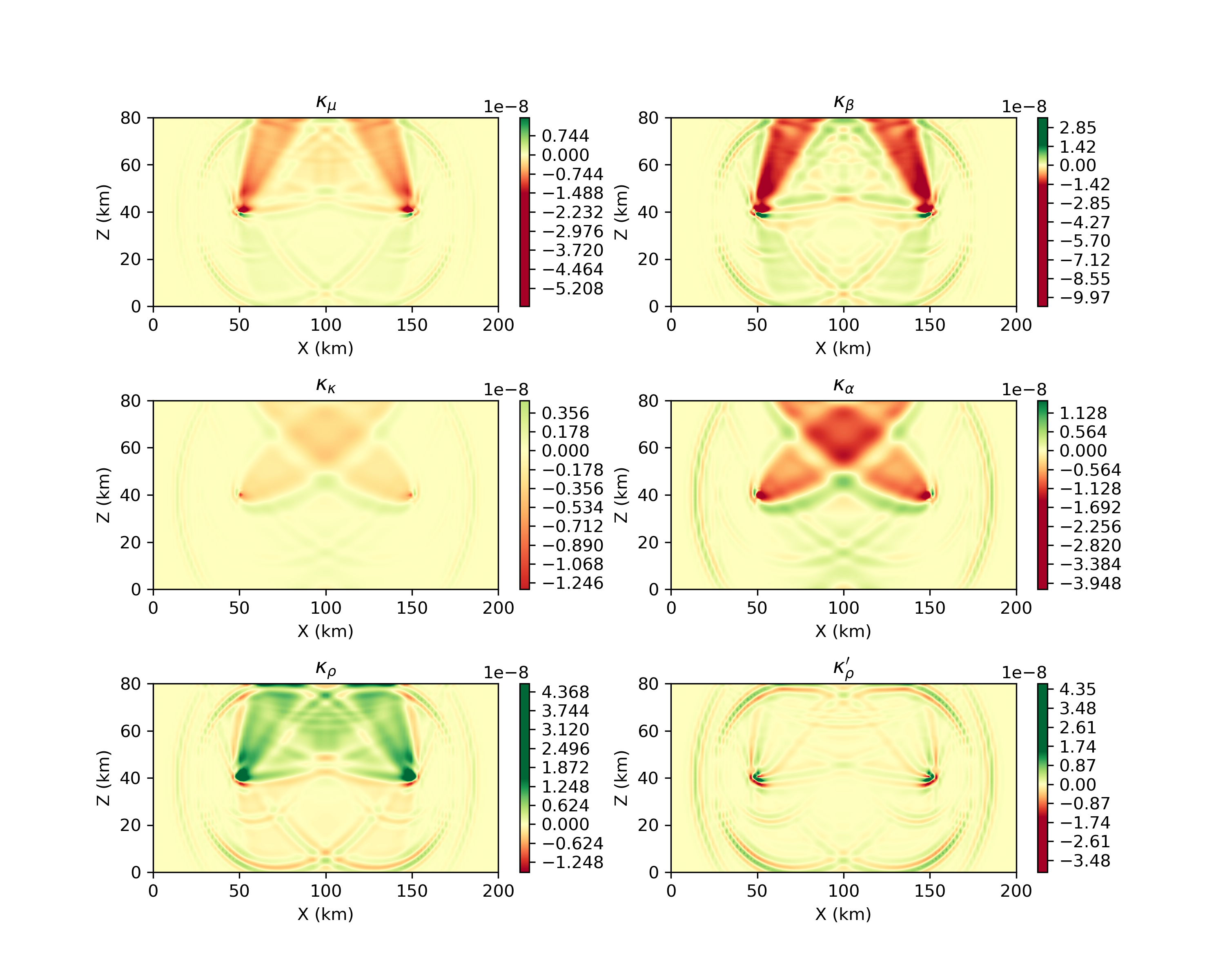
Kernels.