Wave propagation through 3D homogeneous media
In this example we simulate wave propagation through a 3-dimensional homogeneous halfspace using a force source.
Setting up your workspace
Let’s start by creating a workspace from where we can run this example.
mkdir -p ~/specfempp-examples/homogeneous-halfspace-single-force
cd ~/specfempp-examples/homogeneous-halfspace-single-force
We also need to check that the SPECFEM++ executable directory is added to the
PATH.
which specfem3d
If the above command returns a path to the specfem3d executable, then the
executable directory is added to the PATH. If not, you need to add the executable
directory to the PATH using the following command.
export PATH=$PATH:<PATH TO SPECFEM++ DIRECTORY/bin>
Note
Make sure to replace <PATH TO SPECFEM++ DIRECTORY/bin> with the
actual path to the SPECFEM++ directory on your system.
Now let’s create the necessary directories to store the input files and output artifacts.
mkdir -p OUTPUT_FILES
mkdir -p OUTPUT_FILES/results
mkdir -p OUTPUT_FILES/DATABASES
mkdir -p DATA
mkdir -p DATA/meshfem3D_files

touch specfem_config.yaml
touch force.yaml
Generating a mesh
To generate the mesh for the homogeneous halfspace we need a mesh parameter file,
Mesh_Par_file, interface files (interfaces.txt and interface1.txt),
and the mesher executable, xmeshfem3D, which should have been compiled during
the installation process.
Note
The 3D mesher is based on the mesher developed for SPECFEM3D Cartesian. More details on the meshing process can be found in the SPECFEM3D Cartesian documentation.
We first define the meshing parameters in a Mesh Parameter file.
Mesh Parameter File
#-----------------------------------------------------------
#
# Meshing input parameters
#
#-----------------------------------------------------------

MESH_A_CHUNK_OF_THE_EARTH        = .false.
CHUNK_MESH_PAR_FILE              = dummy.txt

# coordinates of mesh block in latitude/longitude and depth in km
LATITUDE_MIN                    = 0.0
LATITUDE_MAX                    = 80000.0
LONGITUDE_MIN                   = 0.0
LONGITUDE_MAX                   = 100000.0
DEPTH_BLOCK_KM                  = 60.d0
UTM_PROJECTION_ZONE             = 11
SUPPRESS_UTM_PROJECTION         = .true.

# file that contains the interfaces of the model / mesh
INTERFACES_FILE                 = DATA/meshfem3D_files/interfaces.txt

# file that contains the cavity
CAVITY_FILE                     = no_cavity.dat

# Number of nodes for 2D and 3D shape functions for hexahedra.
# We use either 8-node mesh elements (bricks) or 27-node elements.
# If you use our internal mesher, the only option is 8-node bricks (27-node elements are not supported).
NGNOD                           = 8

# number of elements at the surface along edges of the mesh at the surface
# (must be 8 * multiple of NPROC below if mesh is not regular and contains mesh doublings)
# (must be multiple of NPROC below if mesh is regular)
NEX_XI                          = 15
NEX_ETA                         = 12

# number of MPI processors along xi and eta (can be different)
NPROC_XI                        = 1
NPROC_ETA                       = 1

#-----------------------------------------------------------
#
# Doubling layers
#
#-----------------------------------------------------------

# Regular/irregular mesh
USE_REGULAR_MESH                = .true.
# Only for irregular meshes, number of doubling layers and their position
NDOUBLINGS                      = 0
# NZ_DOUBLING_1 is the parameter to set up if there is only one doubling layer
# (more doubling entries can be added if needed to match NDOUBLINGS value)
NZ_DOUBLING_1                   = 40
NZ_DOUBLING_2                   = 48

#-----------------------------------------------------------
#
# Visualization
#
#-----------------------------------------------------------

# create mesh files for visualisation or further checking
CREATE_ABAQUS_FILES             = .false.
CREATE_DX_FILES                 = .false.
CREATE_VTK_FILES                = .true.

# stores mesh files as cubit-exported files into directory MESH/ (for single process run)
SAVE_MESH_AS_CUBIT              = .false.

# path to store the databases files
LOCAL_PATH                      = OUTPUT_FILES/DATABASES

#-----------------------------------------------------------
#
# CPML
#
#-----------------------------------------------------------

# CPML perfectly matched absorbing layers
THICKNESS_OF_X_PML              = 12.3d0
THICKNESS_OF_Y_PML              = 12.3d0
THICKNESS_OF_Z_PML              = 12.3d0

#-----------------------------------------------------------
#
# Domain materials
#
#-----------------------------------------------------------

# number of materials
NMATERIALS                      = 1
# define the different materials in the model as:
# #material_id  #rho  #vp  #vs  #Q_Kappa  #Q_mu  #anisotropy_flag  #domain_id
#     Q_Kappa          : Q_Kappa attenuation quality factor
#     Q_mu             : Q_mu attenuation quality factor
#     anisotropy_flag  : 0 = no anisotropy / 1,2,... check the implementation in file aniso_model.f90
#     domain_id        : 1 = acoustic / 2 = elastic
1   2300.0   2800.0   1500.0  0 0 0 2

#-----------------------------------------------------------
#
# Domain regions
#
#-----------------------------------------------------------

# number of regions
NREGIONS                        = 1
# define the different regions of the model as :
#NEX_XI_BEGIN  #NEX_XI_END  #NEX_ETA_BEGIN  #NEX_ETA_END  #NZ_BEGIN #NZ_END  #material_id
1              15           1               12            1         9        1
At this point, it is worthwhile to note a few key parameters within the
Mesh_Par_file as it pertains to SPECFEM++.
This version of SPECFEM++ does not support simulations running across multiple cores/nodes, i.e., we have not enabled MPI. Relevant parameter values:
37NPROC_XI                        = 1
38NPROC_ETA                       = 1
The mesh domain is defined by the coordinates and depth. In this case we define a domain that is 100km x 80km x 60km. Relevant parameter values:
11LATITUDE_MIN                    = 0.0
12LATITUDE_MAX                    = 80000.0
13LONGITUDE_MIN                   = 0.0
14LONGITUDE_MAX                   = 100000.0
15DEPTH_BLOCK_KM                  = 60.d0
16UTM_PROJECTION_ZONE             = 11
17SUPPRESS_UTM_PROJECTION         = .true.
The number of elements along the XI and ETA directions define the horizontal resolution of the mesh:
33NEX_XI                          = 15
34NEX_ETA                         = 12
The path to the interfaces file is provided using the
INTERFACES_FILEparameter:20INTERFACES_FILE = DATA/meshfem3D_files/interfaces.txt
We define a single homogeneous material with density 2300 kg/m³, Vp = 2800 m/s, and Vs = 1500 m/s. The domain type is set to 2 (elastic):
90NMATERIALS                      = 1
91# define the different materials in the model as:
92# #material_id  #rho  #vp  #vs  #Q_Kappa  #Q_mu  #anisotropy_flag  #domain_id
93#     Q_Kappa          : Q_Kappa attenuation quality factor
94#     Q_mu             : Q_mu attenuation quality factor
95#     anisotropy_flag  : 0 = no anisotropy / 1,2,... check the implementation in file aniso_model.f90
96#     domain_id        : 1 = acoustic / 2 = elastic
971   2300.0   2800.0   1500.0  0 0 0 2
We define a single region that spans the entire mesh and assigns material 1 to it:
106NREGIONS                        = 1
107# define the different regions of the model as :
108#NEX_XI_BEGIN  #NEX_XI_END  #NEX_ETA_BEGIN  #NEX_ETA_END  #NZ_BEGIN #NZ_END  #material_id
1091              15           1               12            1         9        1
Interfaces file
The interfaces file defines the topography and layer structure of the mesh.
# number of interfaces
 1
#
# We describe each interface below, structured as a 2D-grid, with several parameters :
# number of points along XI and ETA, minimal XI ETA coordinates
# and spacing between points which must be constant.
# Then the records contain the Z coordinates of the NXI x NETA points.
#
# interface number 1 (topography, top of the mesh)
 .true. 2 2 0.0 0.0 1000.0 1000.0
 DATA/meshfem3D_files/interface1.txt
#
# for each layer, we give the number of spectral elements in the vertical direction
#
# layer number 1 (top layer)
 9
The interfaces file describes:
The number of interfaces (in this case, 1 - the top surface)
For each interface: whether it’s defined by a file (.true.), the number of points along XI and ETA directions, the starting coordinates (0.0, 0.0), and spacing (1000.0, 1000.0)
The path to the interface data file
The number of spectral elements in the vertical direction for each layer (9 elements)
Interface data file
The interface data file contains the elevation values at the grid points:
0
0
0
0
In this case, all elevation values are 0, meaning we have a flat top surface.
Running xmeshfem3D
To execute the mesher run:
xmeshfem3D -p DATA/meshfem3D_files/Mesh_Par_file
Check the mesher generated files in the OUTPUT_FILES/DATABASES directory:
ls -ltr OUTPUT_FILES/DATABASES
You should see files including:
proc000000_Database.bin- the mesh databaseproc000000_mesh.vtk- mesh visualization fileproc000000_skewness.vtk- mesh quality visualization file
Defining receivers (stations)
In 3D simulations, we need to explicitly define the receiver locations using a STATIONS file.
X55 DB 40000.00 55000.00 0.0 0.0
X60 DB 41000.00 60000.00 0.0 0.0
X65 DB 42000.00 65000.00 0.0 0.0
X70 DB 44000.00 70000.00 0.0 0.0
X75 DB 46000.00 75000.00 0.0 0.0
X80 DB 49000.00 80000.00 0.0 0.0
X85 DB 52000.00 85000.00 0.0 0.0
X90 DB 56000.00 90000.00 0.0 0.0
X95 DB 60000.00 95000.00 0.0 0.0
Each line defines a station with the format:
STATION_NAME NETWORK_CODE X Y ELEVATION BURIAL
where:
X, Y are the horizontal coordinates in the mesh coordinate system
ELEVATION is the height above the surface (typically 0.0)
BURIAL is the depth below the surface (typically 0.0)
In this example, we have 9 stations distributed across the domain.
Defining sources
Next we define the sources using a YAML file. For a full description of parameters used to define sources refer to Source Description.
number-of-sources: 1
sources:
  - force:
      x : 51000.0
      y : 43000.0
      z : -31000.0
      source_surf: false
      fx : 0.0
      fy : 0.0
      fz : 1e14
      Ricker:
        factor: 1.0
        tshift: 0.0
        f0: 0.15
In this file, we define a single force source with:
Position: x=51000m, y=43000m, z=-31000m (note: negative z is depth)
Force components: fx=0, fy=0, fz=1e14 (vertical force)
Source time function: Ricker wavelet with center frequency 0.15 Hz
Configuring the solver
Now that we have generated a mesh and defined the sources and receivers, we need to
set up the solver. We define the configuration in a YAML file specfem_config.yaml.
For a full description of parameters refer to SPECFEM++ Parameter Documentation.
parameters:

  header:
    ## Header information is used for logging. It is good practice to give your simulations explicit names
    title: Isotropic Elastic simulation # name for your simulation
    # A detailed description for your simulation
    description: |
      Material systems : Elastic domain (1)
      Interfaces : None
      Sources : Force source (1)
      Boundary conditions : Neumann BCs on all edges

  simulation-setup:
    ## quadrature setup
    quadrature:
      quadrature-type: GLL4

    ## Solver setup
    solver:
      time-marching:
        time-scheme:
          type: Newmark
          dt: 0.16
          nstep: 250

    simulation-mode:
      forward:
        writer:
          seismogram:
            format: "ascii"
            directory: "OUTPUT_FILES/results"

          # display:
          #   format: VTKHDF
          #   directory: OUTPUT_FILES/
          #   field: displacement
          #   component: z
          #   simulation-field: forward
          #   time-interval: 5

  receivers:
    stations: "DATA/STATIONS"
    angle: 0.0
    seismogram-type:
      - displacement
    nstep_between_samples: 1

  ## Runtime setup
  run-setup:
    number-of-processors: 1
    number-of-runs: 1

  ## databases
  databases:
    mesh-database: "OUTPUT_FILES/DATABASES/proc000000_Database.bin"

  ## sources
  sources: "force.yaml"
At this point let’s focus on a few sections in this file:
Configure the solver using the
simulation-setupsection:specfem_config.yaml¶13 simulation-setup: 14 ## quadrature setup 15 quadrature: 16 quadrature-type: GLL4 17 18 ## Solver setup 19 solver: 20 time-marching: 21 time-scheme: 22 type: Newmark 23 dt: 0.16 24 nstep: 250 25 26 simulation-mode: 27 forward: 28 writer: 29 seismogram: 30 format: "ascii" 31 directory: "OUTPUT_FILES/results"
We define the integration quadrature to be used in the simulation (
GLL4)Define the time-stepping scheme (Newmark), time step (0.16s), and number of steps (250)
Set the output format for seismograms to ASCII
Define receiver (station) configuration:
specfem_config.yaml¶41 receivers: 42 stations: "DATA/STATIONS" 43 angle: 0.0 44 seismogram-type: 45 - displacement 46 nstep_between_samples: 1
Specify the path to the STATIONS file
Set the seismogram type to displacement
Set the sampling rate (nstep_between_samples=1 means sample every time step)
Define the path to the mesh database and source description file:
specfem_config.yaml¶54 databases: 55 mesh-database: "OUTPUT_FILES/DATABASES/proc000000_Database.bin" 56 57 ## sources 58 sources: "force.yaml"
Running the solver
Finally, to run the SPECFEM++ solver:
specfem3d -p specfem_config.yaml
Note
Make sure either you are in the executable directory of SPECFEM++ or the
executable directory is added to your PATH.
The solver will output progress information to the terminal and write seismograms
to the OUTPUT_FILES/results directory.
Visualizing seismograms
Let us now plot the source-station geometry and the traces generated by the solver. The following Python script reads the ASCII seismogram files and creates two separate plots:
Source-station geometry with distance circles
Seismograms for each component (MXX, MXY, MXZ) sorted by epicentral distance
  1import numpy as np
  2import matplotlib.pyplot as plt
  3import matplotlib.gridspec as gridspec
  4import glob
  5import yaml
  6from matplotlib.patches import Circle
  7
  8
  9def read_stations(filename):
 10    """Read STATIONS file"""
 11    stations = []
 12    with open(filename, "r") as f:
 13        for line in f:
 14            if line.strip():
 15                parts = line.strip().split()
 16                station = parts[0]
 17                network = parts[1]
 18                y = float(parts[2])  # latitude/UTM_Y
 19                x = float(parts[3])  # longitude/UTM_X
 20                elevation = float(parts[4])
 21                burial = float(parts[5])
 22                stations.append(
 23                    {
 24                        "station": station,
 25                        "network": network,
 26                        "x": x,
 27                        "y": y,
 28                        "elevation": elevation,
 29                        "burial": burial,
 30                    }
 31                )
 32    return stations
 33
 34
 35def read_yaml_source(filename):
 36    """Read source parameters from YAML file"""
 37    with open(filename, "r") as f:
 38        data = yaml.safe_load(f)
 39    source_params = data["sources"][0]["force"]
 40    source = {
 41        "x": source_params["x"],
 42        "y": source_params["y"],
 43        "z": source_params["z"],
 44    }
 45    return source
 46
 47
 48def read_seismogram(filename):
 49    """Read seismogram file"""
 50    data = np.loadtxt(filename)
 51    return data[:, 0], data[:, 1]  # time, displacement
 52
 53
 54def calculate_epicentral_distance(station_x, station_y, source_x, source_y):
 55    """Calculate epicentral distance"""
 56    return np.sqrt((station_x - source_x) ** 2 + (station_y - source_y) ** 2)
 57
 58
 59def main():
 60    # Read station and source data
 61    stations = read_stations("DATA/STATIONS")
 62    source = read_yaml_source("force.yaml")
 63
 64    # Calculate epicentral distances and sort stations
 65    for station in stations:
 66        station["distance"] = calculate_epicentral_distance(
 67            station["x"], station["y"], source["x"], source["y"]
 68        )
 69
 70    stations_sorted = sorted(stations, key=lambda x: x["distance"])
 71
 72    # ========================================
 73    # Figure 1: Source-Station Geometry
 74    # ========================================
 75    fig1 = plt.figure(figsize=(8, 8))
 76    ax1 = fig1.add_subplot(111)
 77
 78    # Plot stations
 79    for station in stations:
 80        ax1.plot(
 81            station["x"],
 82            station["y"],
 83            "rv",
 84            markersize=8,
 85            label="Stations" if station == stations[0] else "",
 86        )
 87        ax1.text(
 88            station["x"],
 89            station["y"] + 1000,
 90            station["station"],
 91            ha="center",
 92            va="bottom",
 93            fontsize=8,
 94        )
 95
 96    # Plot source
 97    ax1.plot(source["x"], source["y"], "r*", markersize=15, label="Source")
 98
 99    # Add circular distance grid
100    max_dist = max([s["distance"] for s in stations])
101    circles = [5000, 10000, 15000, 20000, 25000, 30000, 35000, 40000]
102    for radius in circles:
103        if radius <= max_dist * 1.2:
104            circle = Circle(
105                (source["x"], source["y"]),
106                radius,
107                fill=False,
108                linestyle="--",
109                alpha=0.3,
110                color="gray",
111            )
112            ax1.add_patch(circle)
113            # Add distance labels
114            ax1.text(
115                source["x"] + radius * 0.7,
116                source["y"] + radius * 0.7,
117                f"{radius / 1000:.0f}km",
118                fontsize=8,
119                alpha=0.7,
120            )
121
122    ax1.set_xlabel("X (UTM)")
123    ax1.set_ylabel("Y (UTM)")
124    ax1.set_title("Source-Station Geometry")
125    ax1.legend()
126    ax1.grid(True, alpha=0.3)
127    ax1.set_aspect("equal")
128
129    plt.savefig("OUTPUT_FILES/geometry.png", dpi=300, bbox_inches="tight")
130    print("Saved source-station geometry plot to OUTPUT_FILES/geometry.png")
131
132    # Find seismogram files (current output)
133    seismogram_files = {
134        "MXX": sorted(glob.glob("OUTPUT_FILES/results/*.S3.MXX.semd")),
135        "MXY": sorted(glob.glob("OUTPUT_FILES/results/*.S3.MXY.semd")),
136        "MXZ": sorted(glob.glob("OUTPUT_FILES/results/*.S3.MXZ.semd")),
137    }
138
139    # Find reference seismogram files
140    reference_seismogram_files = {
141        "MXX": sorted(glob.glob("reference_seismograms/*.S3.MXX.semd")),
142        "MXY": sorted(glob.glob("reference_seismograms/*.S3.MXY.semd")),
143        "MXZ": sorted(glob.glob("reference_seismograms/*.S3.MXZ.semd")),
144    }
145
146    # Read all seismograms and find common time range
147    all_seismograms = {}
148    reference_seismograms = {}
149    time_range = None
150    max_displacement = 0
151
152    for component in ["MXX", "MXY", "MXZ"]:
153        all_seismograms[component] = {}
154        reference_seismograms[component] = {}
155
156        # Read current output seismograms
157        for filename in seismogram_files[component]:
158            # Extract station name from filename
159            station_name = filename.split("/")[-1].split(".")[1]
160            time, displacement = read_seismogram(filename)
161            all_seismograms[component][station_name] = (time, displacement)
162
163            # Update global ranges
164            if time_range is None:
165                time_range = (time.min(), time.max())
166            else:
167                time_range = (
168                    min(time_range[0], time.min()),
169                    max(time_range[1], time.max()),
170                )
171            max_displacement = max(max_displacement, np.abs(displacement).max())
172
173        # Read reference seismograms
174        for filename in reference_seismogram_files[component]:
175            # Extract station name from filename
176            station_name = filename.split("/")[-1].split(".")[1]
177            time, displacement = read_seismogram(filename)
178            reference_seismograms[component][station_name] = (time, displacement)
179
180            # Update global ranges
181            if time_range is None:
182                time_range = (time.min(), time.max())
183            else:
184                time_range = (
185                    min(time_range[0], time.min()),
186                    max(time_range[1], time.max()),
187                )
188            max_displacement = max(max_displacement, np.abs(displacement).max())
189
190    # ========================================
191    # Figure 2: Seismograms
192    # ========================================
193    fig2 = plt.figure(figsize=(15, 6))
194    gs = gridspec.GridSpec(1, 3, hspace=0.3, wspace=0.3)
195
196    # Plot seismograms for each component
197    components = ["MXX", "MXY", "MXZ"]
198
199    for i, component in enumerate(components):
200        ax = fig2.add_subplot(gs[0, i])
201
202        # Plot seismograms sorted by epicentral distance
203        y_spacing = max_displacement * 2.5
204
205        for j, station in enumerate(stations_sorted):
206            station_name = station["station"]
207
208            # Plot current output seismogram
209            if station_name in all_seismograms[component]:
210                time, displacement = all_seismograms[component][station_name]
211
212                # Normalize and offset displacement
213                normalized_disp = displacement / max_displacement * y_spacing * 0.8
214                y_pos = j * y_spacing
215
216                ax.plot(
217                    time,
218                    normalized_disp + y_pos,
219                    "k-",
220                    linewidth=0.8,
221                    label="specfem++" if j == 0 else "",
222                )
223
224            # Plot reference seismogram
225            if station_name in reference_seismograms[component]:
226                time_ref, displacement_ref = reference_seismograms[component][
227                    station_name
228                ]
229
230                # Normalize and offset displacement
231                normalized_disp_ref = (
232                    displacement_ref / max_displacement * y_spacing * 0.8
233                )
234                y_pos = j * y_spacing
235
236                ax.plot(
237                    time_ref,
238                    normalized_disp_ref + y_pos,
239                    "r--",
240                    linewidth=0.8,
241                    alpha=0.7,
242                    label="xspecfem3D" if j == 0 else "",
243                )
244
245            # Add station label and distance
246            if (
247                station_name in all_seismograms[component]
248                or station_name in reference_seismograms[component]
249            ):
250                ax.text(
251                    time_range[0] - (time_range[1] - time_range[0]) * 0.05,
252                    y_pos,
253                    f"{station_name}\n({station['distance'] / 1000:.1f}km)",
254                    ha="right",
255                    va="center",
256                    fontsize=8,
257                )
258
259        ax.set_xlabel("Time (s)")
260        ax.set_title(f"Component {component}")
261        ax.set_xlim(time_range)
262        ax.grid(True, alpha=0.3)
263
264        # Add legend for the first component only
265        if i == 0:
266            ax.legend(loc="upper left", fontsize=8, fancybox=False)
267
268        # Set y-axis limits to show all traces properly
269        if len(stations_sorted) > 0:
270            ax.set_ylim(
271                -y_spacing * 0.5,
272                (len(stations_sorted) - 1) * y_spacing + y_spacing * 0.5,
273            )
274
275        # Remove y-tick labels since they're just offsets
276        ax.set_yticklabels([])
277
278        # Set aspect ratio for seismogram plots to be consistent
279        ax.set_aspect("auto")
280
281    plt.savefig("OUTPUT_FILES/seismograms.png", dpi=300, bbox_inches="tight")
282    print("Saved seismograms plot to OUTPUT_FILES/seismograms.png")
283
284    plt.show(block=False)
285
286
287if __name__ == "__main__":
288    main()
To run the plotting script:
python plot_seismograms.py
This will create two plots in the OUTPUT_FILES directory:
geometry.png- showing the source-station geometryseismograms.png- showing the recorded seismograms for all three displacement components

Source-station geometry. The source is marked by a red star and stations by red triangles. Concentric circles indicate epicentral distances in kilometers.

Seismograms recorded at stations distributed across the homogeneous halfspace. The three panels show displacement components (MXX, MXY, MXZ), with traces sorted by epicentral distance from top to bottom.
[Optional] Visualizing the wavefield
To visualize the wavefield propagation through the homogeneous halfspace, we
have a couple of prerequisites. First, SPECFEM++ must be built with VTK and
HDF5 support. Second, Paraview (https://www.paraview.org/) needs to be installed
on your system to visualize the output files. Once these prerequisites are met,
we can uncomment display section in the specfem_config.yaml file to
include the following configuration:
display:
  format: VTKHDF
  directory: OUTPUT_FILES/
  field: displacement
  component: z
  simulation-field: forward
  time-interval: 5
Rerun the solver with the updated configuration. Then open Paraview and load the
generated VTK files from the OUTPUT_FILES directory to visualize the wavefield
propagation.
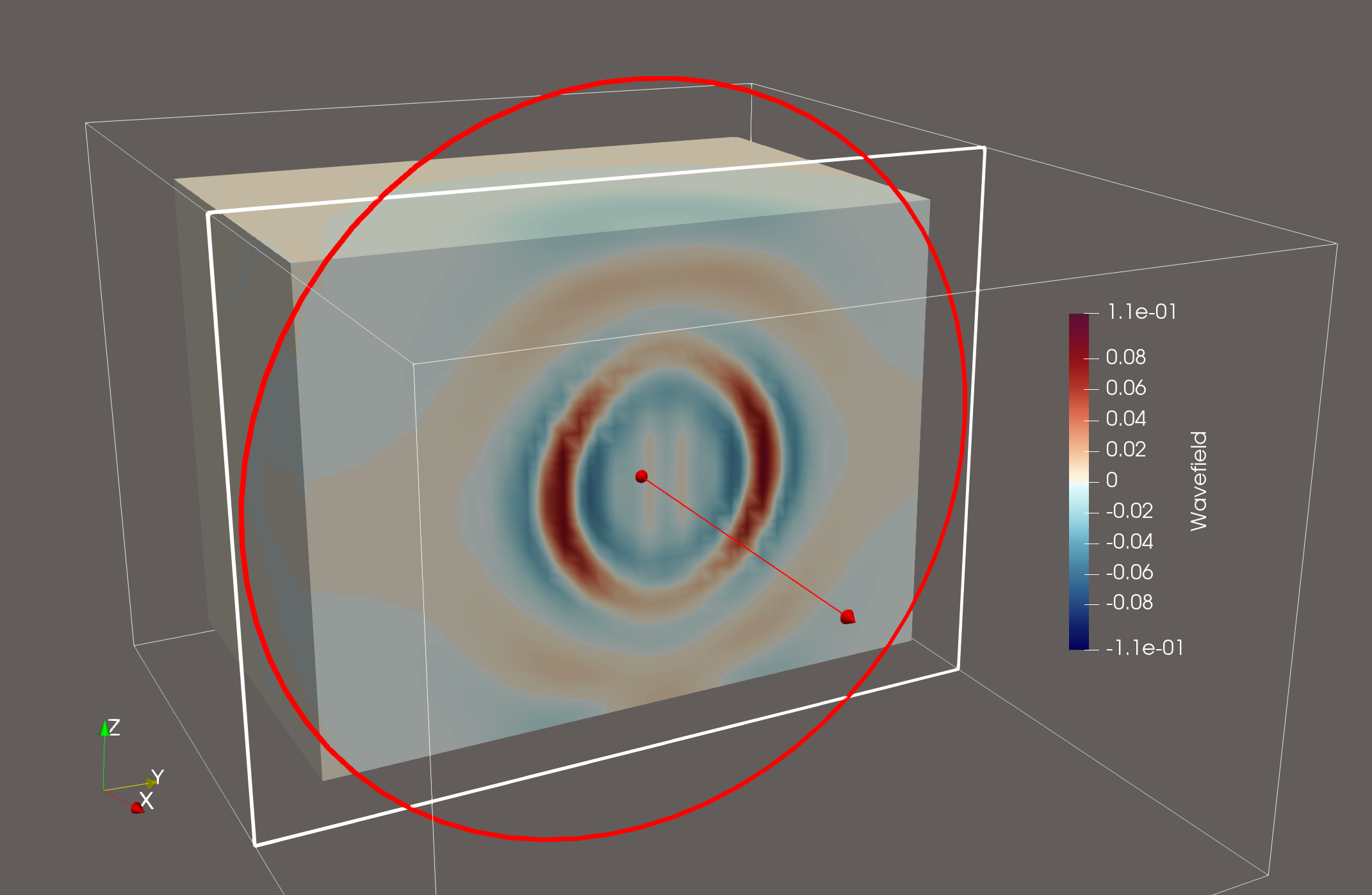
Snapshot of the vertical displacement wavefield propagating through the homogeneous halfspace at a given time step. We sliced the cube halfway along the X-axis to visualize the wavefield inside the volume.