Running SPECFEM++ using a CUBIT mesh¶

As with any finite element solver, SPECFEM++ solver requires a mesh generation step to discritize the domain. In particular, our spectral element solver requires an hexahedral mesh, and does not support tetrahedral meshes. Up until now, all previous examples use the internal mesher to mesh simple domains - particularly domains with layered sandwitch structures. However, for more complex domains, we need to use an external mesher. In this example, we will use CUBIT to generate a mesh for a simple 2D rectangular domain with an ellipsoidal cavity.

Note

Please note that this is not inteded to be an in-depth tutorial on meshing using CUBIT. The goal of this cookbook is to demonstrate how to define the mesh so that SPECFEM++ solver is able to read it. For more information on meshing using CUBIT, please refer to the CUBIT tutorials.`

Creating the domain¶

Let’s start by creating the domain using CUBIT in 5 steps:

Create a rectangular domain with dimensions 200m x 80m
Move the origin to the corner of the rectangle
Create an ellipsoidal cavity with semi-major and semi-minor axes of 40m and 20m respectively
Move the ellipse by (70m, 25m)
Subtract the ellipse from the rectangle to create a cavity

The following script performs the above steps in CUBIT. You can copy and paste this script into the CUBIT command line interface to create the domain.

cubit_script.jou¶

create surface rectangle width 200 height 80 yplane
move Surface 1 x 100 y 0 z 40 include_merged
create surface ellipse major radius 40 minor radius 20 yplane
move Surface 2 x 70 y 0 z 25 include_merged
subtract surface 2 from surface 1

At this point, you’ll notice that your view point is not along the correct axis. You can fix this by changing the view plane within the display drop-down menu.

Note

Please note that you can also create the domain interactively using the CUBIT GUI. Specifically the geometry tab within the command panel.

Meshing the domain¶

Let us now mesh the domain interactively using the CUBIT GUI.

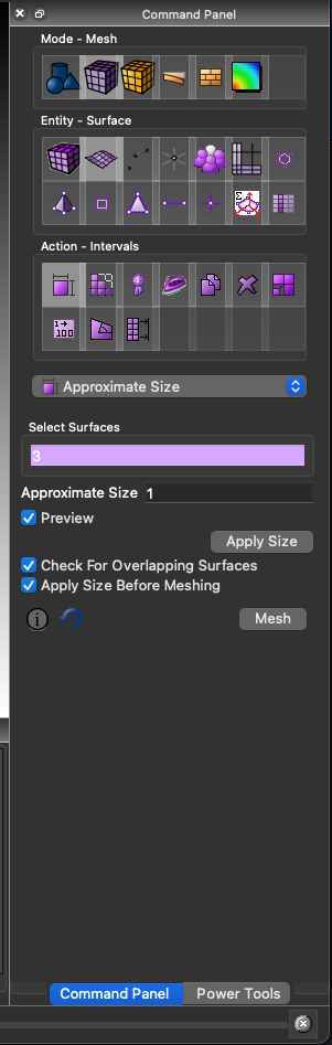
Step 1: Set the mesh size. Here we are setting the approximate size setting to 1, and select_surfaces to 3. Make sure to click apply size bottom after setting the size.
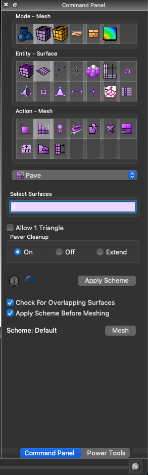
Step 2: Generate the mesh. Set the select_surfaces to 3. Click the mesh button after selecting the pave setting.

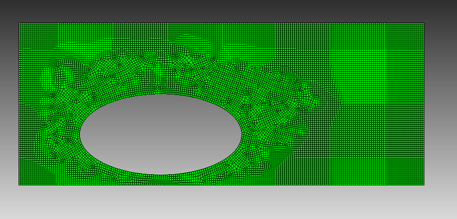
The final mesh should look similar to the one below. You should have ~13500 elements within the mesh.

Generating blocks to be read by SPECFEM++¶

Blocks within CUBIT are a collection of mesh elements that have common properties. For the mesh we are generating we need to generate 5 blocks.

Block 1: A material block for the solid medium which contains all elements within the mesh.

material_block_1.jou¶

block 1 face in surf 3
block 1 name 'Granit'
block 1 element type QUAD4
block 1 attribute count 1 ## This attribute defines the material from the par file associated with this block

Note

It is important that we create the material block with a face attribute. This is used as a reference to identify the block within the export script we’ll use later.

Block 2: An absorbing boundary block for the bottom boundary

absorbing_block_2.jou¶

block 2 edge in curve 1
block 2 name 'abs_bottom'
block 2 element type BAR2

Block 3: An absorbing boundary block for the left boundary

absorbing_block_3.jou¶

block 3 edge in curve 2
block 3 name 'abs_left'
block 3 element type BAR2

Block 4: An absorbing boundary block for the top boundary

absorbing_block_3.jou¶

block 4 edge in curve 3
block 4 name 'abs_top'
block 4 element type BAR2

Block 5: An absorbing boundary block for the right boundary

absorbing_block_5.jou¶

block 5 edge in curve 4
block 5 name 'abs_right'
block 5 element type BAR2

Exporting the mesh¶

Exporting the mesh requires running a python script that is available within the SPECFEM++ repository. You can find the script at <PATH TO SPECFEM++ DIRECTORY>/scripts/CUBIT/export_cubit.py.

import_script.jou¶

play "<PATH TO SPECFEM++ DIRECTORY>/scripts/CUBIT/export_cubit.py"

Make sure to replace <PATH TO SPECFEM++ DIRECTORY> with the actual path to the SPECFEM++ directory on your system. Next we need to switch to a directory where we want to export the mesh. To do set the working directory to <PATH TO WORKING DIRECTORY> using file drop-down menu within the command panel.

Finally, we can export the mesh using the export2SPECFEM2D python function defined in the above python script.

Note

Make sure to switch to python tab within the command line panel.

export_script.jou¶

export2SPECFEM2D()

This should generate the following files within the working directory.

mesh_file - File containing the connectivity of the mesh
nodes_coord_file - File containing the coordinates of the mesh nodes
free_surface_file - File containing the nodes on the free surface
absorbing_surface_file - File containing the nodes on the absorbing boundaries
material_file - File containing the material properties for each element

Running the Mesher¶

Now let’s define the meshing parameters in a parameter file, and run the mesher to generate the database.

We now define the CUBIT generated files in the following lines

We can now run the mesher using the following command.

xmeshfem2D -p Par_file

Running the solver¶

As we did in all previous examples, we need to now define the sources and simulation parameters in the following files.

sources.yaml - File containing the source parameters

sources.yaml¶

number-of-sources: 1
sources:
  - force:
      x : 150.0
      z : 40.0
      source_surf: false
      angle : 0.0
      vx : 0.0
      vz : 0.0
      Ricker:
        factor: 1e10
        tshift: 0.0
        f0: 1000.0

specfem_config.yaml - File containing the simulation parameters

specfem_config.yaml¶

## Coupling interfaces have code flow that is dependent on orientation of the interface.
## This test is to check the code flow for horizontal acoustic-elastic interface with acoustic domain on top.

parameters:

  header:
    ## Header information is used for logging. It is good practice to give your simulations explicit names
    title: CUBIT mesh (Homogeneous elastic domains with a cavity)
    # A detailed description for your simulation
    description: |
      Material systems : Elastic domain (1)
      Interfaces : None
      Sources : Force source (1)
      Boundary conditions : Neumann BCs on all edges

  simulation-setup:
    ## quadrature setup
    quadrature:
      quadrature-type: GLL4

    ## Solver setup
    solver:
      time-marching:
        type-of-simulation: forward
        time-scheme:
          type: Newmark
          dt: 2.5e-6
          nstep: 10000

    simulation-mode:
      forward:
        writer:
          seismogram:
            format: ascii
            directory: "OUTPUT_FILES/results"
          display:
            format: PNG
            directory: "OUTPUT_FILES/display"
            field: displacement
            simulation-field: forward
            time-interval: 100

  receivers:
    stations: "OUTPUT_FILES/STATIONS"
    angle: 0.0
    seismogram-type:
      - displacement
    nstep_between_samples: 1

  ## Runtime setup
  run-setup:
    number-of-processors: 1
    number-of-runs: 1

  ## databases
  databases:
    mesh-database: "OUTPUT_FILES/database.bin"

  ## sources
  sources: "sources.yaml"

Finally, we can run the solver using the following command.

specfem2D -p specfem_config.yaml

[Optional] Visualizing the wavefield¶

To create an animated gif of the wavefield evolution, you can use ImageMagick (if available):

magick OUTPUT_FILES/display/wavefield*.png -trim +repage -delay 10 -loop 0 wavefield.gif

The output animated gif will show the wavefield evolution over time. We can see that the P-wave is impinging on the cavity diffracting/reflecting along the edge, and a little later the S-wave doing the same with the addition of S-to-P reflections.