Wave propagation through solid-solid interface
In this example (see benchmarks/src/dim2/solid-solid-interface) we are simulating a medium with two solids. This is a classic
example from the computational seismology class at Princeton University, in which
students are familiarized with wave propagation through an elastic medium.
The model that we are using is a 2D model with a solid-solid interface. The characteristics of the medium are shown in the figure below.
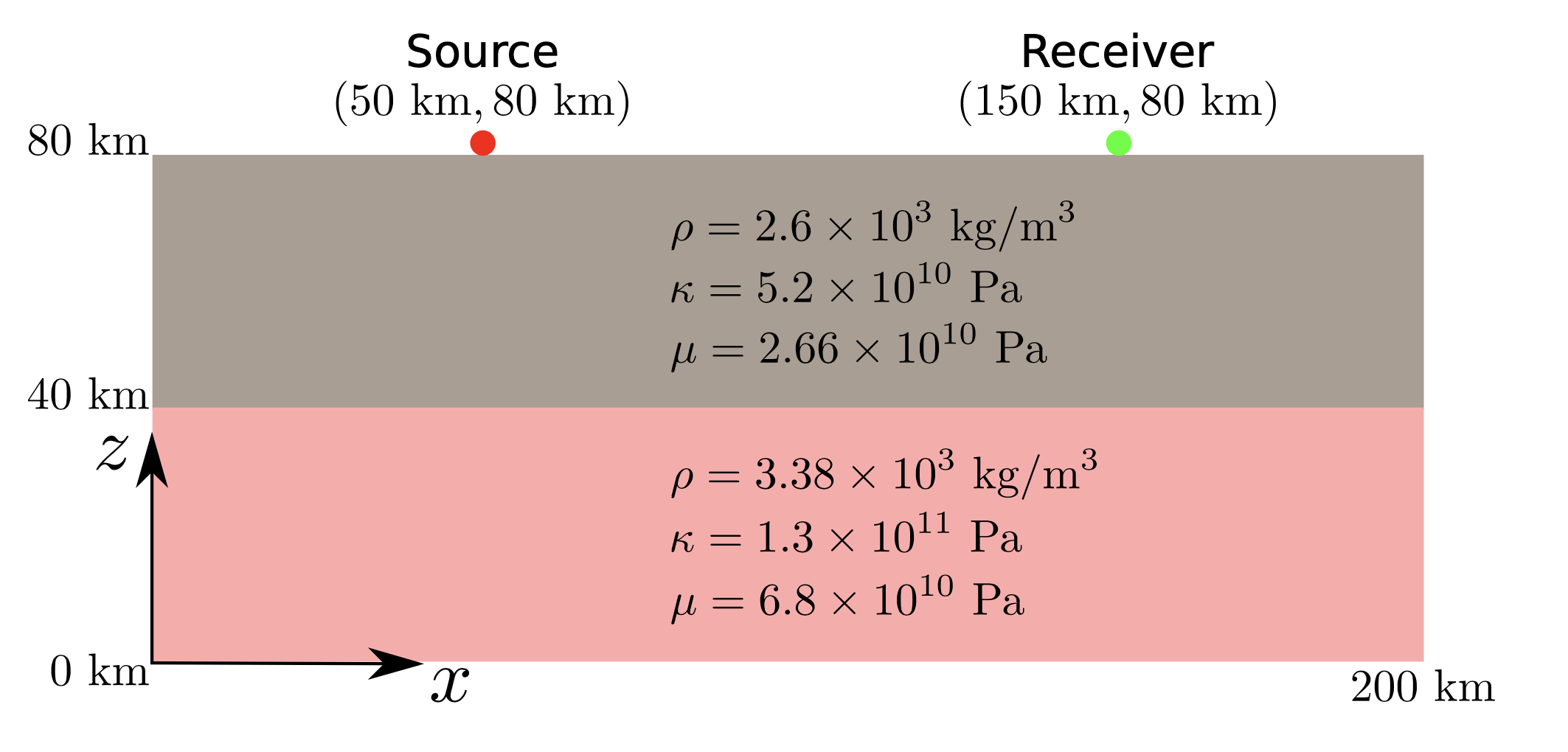
Solid-solid interface model with a slow material on top and a fast material at the bottom.
The model consists of two materials, one with a slower velocity and the other with a faster velocity. The model is divided by a horizontal interface. The source and the receiver are both indicated in the figure and located at the surface of the model.
We will model wave propagation for both P-SV and SH polarized elastic waves in the above model.
Setting up the workspace
Let’s start by creating a workspace from where we can run this example.
mkdir -p ~/specfempp-examples/solid-solid-interface
cd ~/specfempp-examples/solid-solid-interface
We also need to check that the SPECFEM++ build directory is added to the PATH.
which specfem2d
If the above command returns a path to the specfem2d executable, then the
build directory is added to the PATH. If not, you need to add the build
directory to the PATH using the following command.
export PATH=$PATH:<PATH TO SPECFEM++ DIRECTORY/bin>
Note
Make sure to replace <PATH TO SPECFEM++ DIRECTORY/bin> with the
actual path to the SPECFEM++ directory on your system.
Now let’s create the necessary directories to store the input files and output artifacts.
mkdir -p OUTPUT_FILES
mkdir -p OUTPUT_FILES/results_psv
mkdir -p OUTPUT_FILES/results_sh

touch specfem_config_psv.yaml
touch specfem_config_sh.yaml
touch sources.yaml
touch topography_file.dat
touch Par_File
Meshing the domain
We first start by generating a mesh for our simulation domain using
xmeshfem2D. To do this, we first define our simulation domain and the
meshing parmeters in a parameter file.
Parameter file
#-----------------------------------------------------------
#
# Simulation input parameters
#
#-----------------------------------------------------------

# title of job
title                           = Flat solid/solid interface

# parameters concerning partitioning
NPROC                           = 1              # number of processes

# Output folder to store mesh related files
OUTPUT_FILES                   = OUTPUT_FILES

#-----------------------------------------------------------
#
# Mesh
#
#-----------------------------------------------------------

# Partitioning algorithm for decompose_mesh
PARTITIONING_TYPE               = 3              # SCOTCH = 3, ascending order (very bad idea) = 1

# number of control nodes per element (4 or 9)
NGNOD                           = 9

# location to store the mesh
database_filename               = OUTPUT_FILES/database.bin

#-----------------------------------------------------------
#
# Receivers
#
#-----------------------------------------------------------

# use an existing STATION file found in ./DATA or create a new one from the receiver positions below in this Par_file
use_existing_STATIONS           = .false.

# number of receiver sets (i.e. number of receiver lines to create below)
nreceiversets                   = 1

# orientation
anglerec                        = 0.d0         # angle to rotate components at receivers
rec_normal_to_surface           = .false.      # base anglerec normal to surface (external mesh and curve file needed)

# first receiver set (repeat these 6 lines and adjust nreceiversets accordingly)
nrec                            = 1             # number of receivers
xdeb                            = 150000.d0     # first receiver x in meters
zdeb                            = 80000.d0      # first receiver z in meters
xfin                            = 150000.d0     # last receiver x in meters (ignored if only one receiver)
zfin                            = 3480000.d0    # last receiver z in meters (ignored if only one receiver)
record_at_surface_same_vertical = .false.       # receivers inside the medium or at the surface

# filename to store stations file
stations_filename              = OUTPUT_FILES/STATIONS

#-----------------------------------------------------------
#
# Velocity and density models
#
#-----------------------------------------------------------

# number of model materials
nbmodels                        = 2
# available material types (see user manual for more information)
#   acoustic:    model_number 1 rho Vp 0  0 0 QKappa Qmu 0 0 0 0 0 0
#   elastic:     model_number 1 rho Vp Vs 0 0 QKappa Qmu 0 0 0 0 0 0
#   anistoropic: model_number 2 rho c11 c13 c15 c33 c35 c55 c12 c23 c25 0 0 0
#   poroelastic: model_number 3 rhos rhof phi c kxx kxz kzz Ks Kf Kfr etaf mufr Qmu
#   tomo:        model_number -1 0 9999 9999 A 0 0 9999 9999 0 0 0 0 0
#
# The problem values are as follows:
# top:    rho = 2.60 * 10^3 kg/m3, kappa= 5.2 * 10^10 Pa, mu =2.66 * 10^10 Pa
# bottom: rho = 3.38 * 10^3 kg/m3, kappa= 1.3 * 10^11 Pa, mu = 6.8 * 10^10 Pa
# After conversion to VP/VS we have following model values.
1 1 3380.d0 8079.98d0 4485.35d0 0 0 9999 9999 0 0 0 0 0 0
2 1 2600.d0 5859.90d0 3199.40d0 0 0 9999 9999 0 0 0 0 0 0

# external tomography file
TOMOGRAPHY_FILE                 = ./DATA/tomo_file.xyz

# use an external mesh created by an external meshing tool or use the internal mesher
read_external_mesh              = .false.

#-----------------------------------------------------------
#
# PARAMETERS FOR EXTERNAL MESHING
#
#-----------------------------------------------------------

# data concerning mesh, when generated using third-party app (more info in README)
# (see also absorbing_conditions above)
mesh_file                       = ./DATA/Mesh_canyon/canyon_mesh_file   # file containing the mesh
nodes_coords_file               = ./DATA/Mesh_canyon/canyon_nodes_coords_file   # file containing the nodes coordinates
materials_file                  = ./DATA/Mesh_canyon/canyon_materials_file   # file containing the material number for each element
free_surface_file               = ./DATA/Mesh_canyon/canyon_free_surface_file   # file containing the free surface
axial_elements_file             = ./DATA/axial_elements_file   # file containing the axial elements if AXISYM is true
absorbing_surface_file          = ./DATA/Mesh_canyon/canyon_absorbing_surface_file   # file containing the absorbing surface
acoustic_forcing_surface_file   = ./DATA/MSH/Surf_acforcing_Bottom_enforcing_mesh   # file containing the acoustic forcing surface
absorbing_cpml_file             = ./DATA/absorbing_cpml_file   # file containing the CPML element numbers
tangential_detection_curve_file = ./DATA/courbe_eros_nodes  # file containing the curve delimiting the velocity model

#-----------------------------------------------------------
#
# PARAMETERS FOR INTERNAL MESHING
#
#-----------------------------------------------------------

# file containing interfaces for internal mesh
interfacesfile                  = topography_file.dat

# geometry of the model (origin lower-left corner = 0,0) and mesh description
xmin                            = 0.d0          # abscissa of left side of the model
xmax                            = 200000.d0     # abscissa of right side of the model
nx                              = 300           # number of elements along X

STACEY_ABSORBING_CONDITIONS    = .true.

# absorbing boundary parameters (see absorbing_conditions above)
absorbbottom                    = .true.
absorbright                     = .true.
absorbtop                       = .false.
absorbleft                      = .true.

# define the different regions of the model in the (nx,nz) spectral-element mesh
nbregions                       = 2              # then set below the different regions and model number for each region
1 300 1   60 1
1 300 61  120 2

#-----------------------------------------------------------
#
# Display parameters
#
#-----------------------------------------------------------

# meshing output
output_grid_Gnuplot             = .false.        # generate a GNUPLOT file containing the grid, and a script to plot it
output_grid_ASCII               = .false.        # dump the grid in an ASCII text file consisting of a set of X,Y,Z points or not
Like we did in the Wave propagation through homogeneous media, we define the elastic velocity model layers in the Velocity and density models section of the parameter file. This time, however, we define two material systems with different elastic parameters as defined in the figure above. First, we adjust the number of model materials to 2 using the
nbmodelsparameter.Par_file¶65nbmodels = 2
Then, we then define the velocity model for each material based on the parameters in the figure above. We define the elastic material using following format
model_number 1 rho Vp Vs 0 0 QKappa Qmu 0 0 0 0 0 0
Since \(\kappa\), \(\mu\) and \(\rho\) are provided by the model we need to convert them to the velocity parameters \(v_p\) and \(v_s\).
\[v_p = \sqrt{\frac{\kappa + 4/3 \mu}{\rho}}\qquad\qquad v_s = \sqrt{\frac{\mu}{\rho}}\]and add them to the
Par_file:Par_file¶771 1 3380.d0 8079.98d0 4485.35d0 0 0 9999 9999 0 0 0 0 0 0 782 1 2600.d0 5859.90d0 3199.40d0 0 0 9999 9999 0 0 0 0 0 0
we set the quality factors \(Q_{\kappa}\) and \(Q_{\mu}\) to 9999 to avoid attenuation in the model.
Additionally, we define stacey absorbing boundary conditions on all the edges of the domain except the top surface using the
STACEY_ABSORBING_CONDITIONS,absorbbottom,absorbright,absorbtopandabsorbleftparameters.Par_file¶118STACEY_ABSORBING_CONDITIONS = .true. 119 120# absorbing boundary parameters (see absorbing_conditions above) 121absorbbottom = .true. 122absorbright = .true. 123absorbtop = .false. 124absorbleft = .true.
We define a single receiver at the surface of the model at \(x=150\mathrm{km}\) and \(z=80\mathrm{km}\) in the
Par_file.Par_file¶40# number of receiver sets (i.e. number of receiver lines to create below) 41nreceiversets = 1 42 43# orientation 44anglerec = 0.d0 # angle to rotate components at receivers 45rec_normal_to_surface = .false. # base anglerec normal to surface (external mesh and curve file needed) 46 47# first receiver set (repeat these 6 lines and adjust nreceiversets accordingly) 48nrec = 1 # number of receivers 49xdeb = 150000.d0 # first receiver x in meters 50zdeb = 80000.d0 # first receiver z in meters 51xfin = 150000.d0 # last receiver x in meters (ignored if only one receiver) 52zfin = 3480000.d0 # last receiver z in meters (ignored if only one receiver) 53record_at_surface_same_vertical = .false. # receivers inside the medium or at the surface 54 55# filename to store stations file 56stations_filename = OUTPUT_FILES/STATIONS
We define one receiver set
nreceiversetsand a single receivernreclocated.
Defining the topography of the domain
We define the bounds and topography of the domain using the following topography file
#
# number of interfaces
#
 3
#
# for each interface below, we give the number of points and then x,z for each point
#
#
# interface number 1 (bottom of the mesh)
#
 2
 0 0
 200000 0
#
# interface number 2 (ocean bottom)
#
 2
 0 40000
 200000 40000
#
# interface number 3 (topography, top of the mesh)
#
 2
 0 80000
 200000 80000
#
# for each layer, we give the number of spectral elements in the vertical direction
#
#
# layer number 1 (bottom layer)
#
## DK DK the original 2000 Geophysics paper used nz = 90 but NGLLZ = 6
## DK DK here I rescale it to nz = 108 and NGLLZ = 5 because nowadays we almost always use NGLLZ = 5
 60
#
# layer number 2 (top layer)
#
 60
With 38 elements vertically in each layer.
Running xmeshfem2D
To execute the mesher run
xmeshfem2D -p Par_File
Note
Make sure either your are in the executable directory of SPECFEM2D kokkos or
the executable directory is added to your PATH.
Note the path of the database file and a stations file generated after successfully running the mesher.
Defining the source
We define the source location and the source time function in the source file.
number-of-sources: 1
sources:
  - force:
      x : 50000.0
      z : 80000.0
      source_surf: false
      angle : 0.0
      vx : 0.0
      vz : 0.0
      dGaussian:
        factor: 1e10
        tshift: 0.0
        f0: 1.5
We define the source at the surface of the model at \(x=50\mathrm{km}\) and \(z=80\mathrm{km}\), with a first derivative of a Gaussian source time function with a dominant frequency of 1.5 Hz.
Running the P-SV simulation
To run the solver, we first need to define a configuration file
specfem_config_psv.yaml. The _psv just to distinguish this
configuration to solve for the P-SV polarized elastic wave propagation from later on
solved SH polarized elastic wave propagation.
## Coupling interfaces have code flow that is dependent on orientation of the interface.
## This test is to check the code flow for horizontal acoustic-elastic interface with acoustic domain on top.

parameters:

  header:
    ## Header information is used for logging. It is good practice to give your simulations explicit names
    title: Heterogeneous elastic-elastic medium with 1 elastic-elastic interface (orientation horizontal)  # name for your simulation
    # A detailed description for your simulation
    description: |
      Material systems : Elastic domain (1), Elastic domain (1)
      Interfaces : Elastic-elastic interface (1) (orientation horizontal slower medium on top)
      Sources : Force source (1)
      Boundary conditions : Neumann BCs on all edges
      Debugging comments: This tests checks coupling elastic-elastic interface implementation.
                          The orientation of the interface is horizontal with elastic domain on top.

  simulation-setup:
    ## Elastic wave propagation setup
    elastic-wave: "P_SV"

    ## quadrature setup
    quadrature:
      quadrature-type: GLL4

    ## Solver setup
    solver:
      time-marching:
        type-of-simulation: forward
        time-scheme:
          type: Newmark
          dt: 9.0e-3
          nstep: 5000

    simulation-mode:
      forward:
        writer:
          seismogram:
            format: ascii
            directory: OUTPUT_FILES/results_psv

          ## Uncomment to enable the storing of snapshots if VTK is enabled
          ## and installed
          # display:
          #   format: PNG
          #   directory: "OUTPUT_FILES/results_psv"
          #   field: velocity
          #   simulation-field: forward
          #   time-interval: 100

  receivers:
    stations: OUTPUT_FILES/STATIONS
    angle: 0.0
    seismogram-type:
      - displacement
    nstep_between_samples: 1

  ## Runtime setup
  run-setup:
    number-of-processors: 1
    number-of-runs: 1

  ## databases
  databases:
    mesh-database: OUTPUT_FILES/database.bin

  ## sources
  sources: sources.yaml
For the specfem_config_psv.yaml file, nothing has changed compared to the
previous example, Wave propagation through homogeneous media. With the configuration file in
place, we can run the solver using the following command
specfem2d -p specfem_config_psv.yaml
A snapshot of the wavefield at timestep 1100 (\(t=9.9\mathrm{s}\)) is shown below.

Snapshot of the wavefield at timestep 1100 (\(t=9.9\mathrm{s}\)).
Note
The wavefield snapshots are currently not being generated with this setup.
The first (P) wavefront in the upper half of the medium reaches the horizontal center of model after 9 seconds, which is intuitive since the P-wave velocity in the upper half of the model is almost \(6\mathrm{km}/\mathrm{s}\).
The seismograms recorded at the receiver location are shown below.
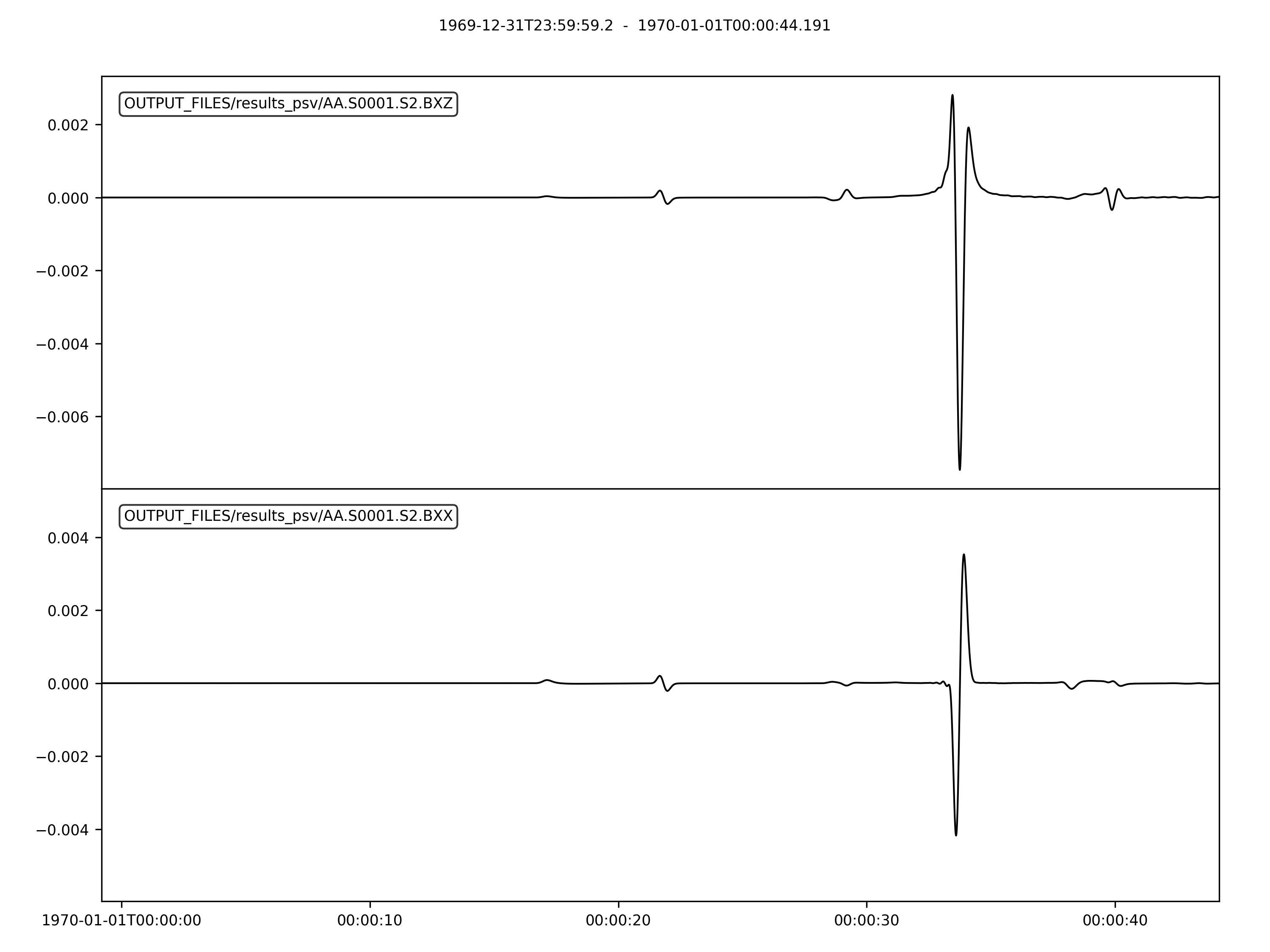
Seismograms recorded at the receiver location.
And the plot can be reproduced using the following python script
import glob
import os
import numpy as np
import obspy

# Set matplotlib gui off
import matplotlib

matplotlib.use("Agg")


def get_traces(directory):
    traces = []
    files = glob.glob(directory + "/*.sem*")
    ## iterate over all seismograms
    for filename in files:
        station_name = os.path.splitext(filename)[0]
        network, station, location, channel = station_name.split(".")[:4]
        trace = np.loadtxt(filename, delimiter=" ")
        starttime = trace[0, 0]
        dt = trace[1, 0] - trace[0, 0]
        traces.append(
            obspy.Trace(
                trace[:, 1],
                {
                    "network": network,
                    "station": station,
                    "location": location,
                    "channel": channel,
                    "starttime": starttime,
                    "delta": dt,
                },
            )
        )

    stream = obspy.Stream(traces)

    return stream


stream = get_traces("OUTPUT_FILES/results_psv")
stream.plot(size=(1000, 750)).savefig("OUTPUT_FILES/seismograms_psv.png", dpi=300)
Running the SH simulation
To run the solver, we first need to define a configuration file
specfem_config_sh.yaml.
## Coupling interfaces have code flow that is dependent on orientation of the interface.
## This test is to check the code flow for horizontal acoustic-elastic interface with acoustic domain on top.

parameters:

  header:
    ## Header information is used for logging. It is good practice to give your simulations explicit names
    title: Heterogeneous elastic-elastic medium with 1 elastic-elastic interface (orientation horizontal)  # name for your simulation
    # A detailed description for your simulation
    description: |
      Material systems : Elastic domain (1), Elastic domain (1)
      Interfaces : Elastic-elastic interface (1) (orientation horizontal slower medium on top)
      Sources : Force source (1)
      Boundary conditions : Neumann BCs on all edges
      Debugging comments: This tests checks coupling elastic-elastic interface implementation.
                          The orientation of the interface is horizontal with elastic domain on top.

  simulation-setup:
    ## Elastic Wave Propagation setup
    elastic-wave: "SH"

    ## quadrature setup
    quadrature:
      quadrature-type: GLL4

    ## Solver setup
    solver:
      time-marching:
        type-of-simulation: forward
        time-scheme:
          type: Newmark
          dt: 9.0e-3
          nstep: 5000

    simulation-mode:
      forward:
        writer:
          seismogram:
            format: ascii
            directory: OUTPUT_FILES/results_sh

          ## Uncomment to enable the storing of snapshots if VTK is enabled
          ## and installed
          # display:
          #   format: PNG
          #   directory: "OUTPUT_FILES/results_sh"
          #   field: velocity
          #   simulation-field: forward
          #   time-interval: 100

  receivers:
    stations: OUTPUT_FILES/STATIONS
    angle: 0.0
    seismogram-type:
      - displacement
    nstep_between_samples: 1

  ## Runtime setup
  run-setup:
    number-of-processors: 1
    number-of-runs: 1

  ## databases
  databases:
    mesh-database: OUTPUT_FILES/database.bin

  ## sources
  sources: sources.yaml
For the specfem_config_sh.yaml file, nothing has changed compared to the
previous example, Wave propagation through homogeneous media. With the configuration file in
place, we can run the solver using the following command
specfem2d -p specfem_config_sh.yaml
A snapshot of the wavefield at timestep 1100 (\(t=9.9\mathrm{s}\)) is shown below.

Snapshot of the wavefield at timestep 1100 (\(t=9.9\mathrm{s}\)).
Note
The wavefield snapshots are currently not being generated with this setup.
The SH wave has still not reach the vertical center of the model after 9.9 seconds, which is intuitive since the SH-wave velocity in the upper half of the model is \(\sim3.2\mathrm{km}/\mathrm{s}\).
To see the SH interacting with the solid-solid interface, we need to run the simulation for a longer time. Here, another snapshot of the wavefield at timestep 2200 (\(t=19.8\mathrm{s}\)) is shown below.

Snapshot of the wavefield at timestep 2200 (\(t=19.8\mathrm{s}\)). The SH wave has now reached the solid-solid interface and is propagating through the model.
The seismograms recorded at the receiver location are shown below.
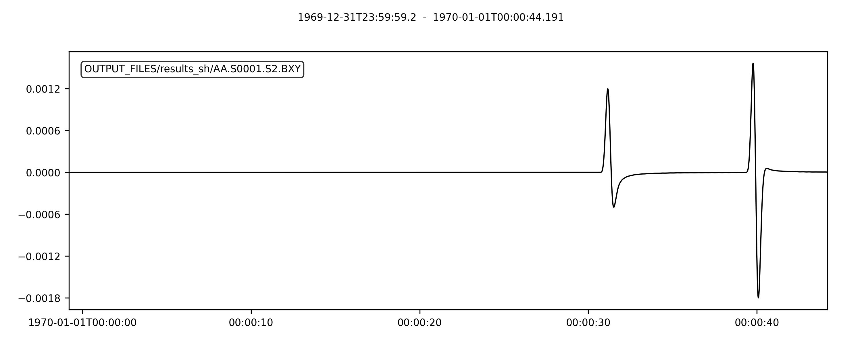
Seismograms recorded at the receiver location.
And the plot can be reproduced using the following python script
import glob
import os
import numpy as np
import obspy

# Set matplotlib gui off
import matplotlib

matplotlib.use("Agg")


def get_traces(directory):
    traces = []
    files = glob.glob(directory + "/*.sem*")
    ## iterate over all seismograms
    for filename in files:
        station_name = os.path.splitext(filename)[0]
        network, station, location, channel = station_name.split(".")[:4]
        trace = np.loadtxt(filename, delimiter=" ")
        starttime = trace[0, 0]
        dt = trace[1, 0] - trace[0, 0]
        traces.append(
            obspy.Trace(
                trace[:, 1],
                {
                    "network": network,
                    "station": station,
                    "location": location,
                    "channel": channel,
                    "starttime": starttime,
                    "delta": dt,
                },
            )
        )

    stream = obspy.Stream(traces)

    return stream


stream = get_traces("OUTPUT_FILES/results_sh")
stream.plot(size=(1000, 400)).savefig("OUTPUT_FILES/seismograms_sh.png", dpi=300)